Decision trees have been widely used in machine learning for classification and regression tasks based on their tree-like structure that represents a series of decisions and their possible consequences. In order to improve the accuracy of decision trees, researchers have proposed a new method called Ant Colony Decision Trees (ACDT), based on the Ant Colony Optimization (ACO). The ACO is a metaheuristic inspired by the foraging behavior of real ants, where they search for the shortest path between their nest and food sources by considering both local heuristics and previous knowledge, observed by pheromone changes. This article will start with introductions of the decision tree and ACO, then expand to the more complex ACDT, including detailed explanations of the algorithm and examples.
Decision Trees
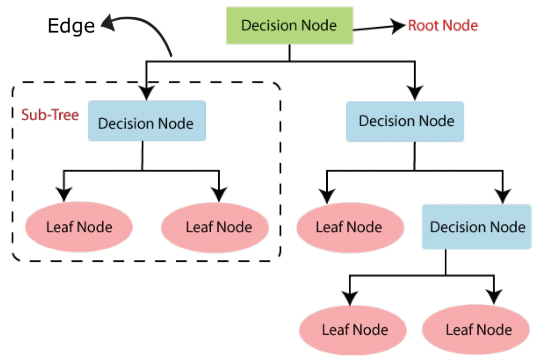
A decision tree is a non-parametric supervised learning algorithm for classification and regression tasks. It has a hierarchical tree structure consisting of a root node, decision nodes, edges, and leaf nodes. It follows an iterative top-down procedure of selecting the best attribute to label an decision node of the tree. It starts at the root node that contains the entire sample, then splits at the decision node that serves as the test condition, and ends at the leaf node that is the final prediction result (Figure 1). This basic approach represents a greedy strategy to create a decision tree since the selection of an attribute at early iterations cannot be reconsidered at later iterations. i.e., the selection of the best attribute is made locally at each iteration, without taking into consideration its influence over the subsequent iterations. However, the newly proposed ACDT algorithm is able to construct the decision tree in a top-down fashion by probabilistically selecting attributes to be added as decision nodes based on the amount of pheromone and heuristics information, with the pheromone values represent the quality of the connection between a parent and child decision nodes.
Ant Colony Optimization (ACO)
Background
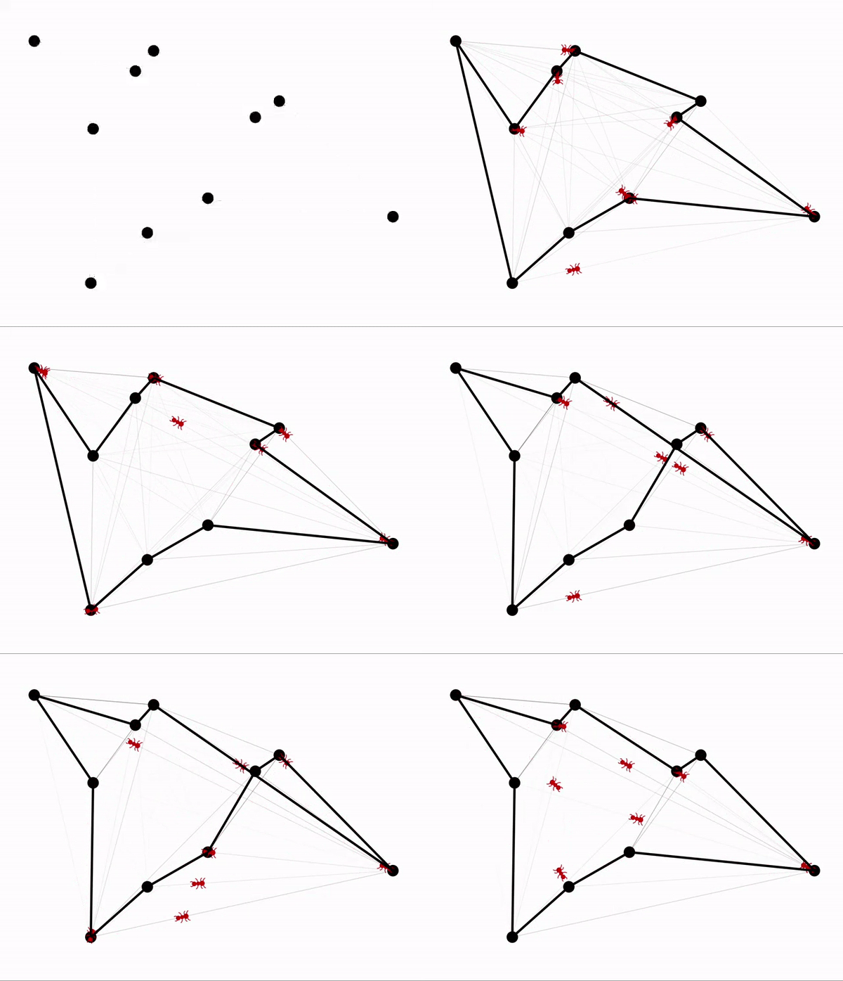
Ant colony optimization (ACO) technique is inspired by the foraging behavior of ant colonies. The intelligent behavior of ant colonies is achieved by making small changes to the environment (i.e., leaving pheromones) in order to communicate indirectly with each other to accomplish complex tasks. When ants leave their colony in search of food, they explore various potential paths from their nest to the targeted food source. Each ant leaves behind a pheromone trail on its path. If a path is selected by multiple ants, it would collect a higher concentration of pheromone. Conversely, if there are no ants continuously following this path, the pheromone deposited by previous ants would evaporate. The concentration of pheromone on each path would affect the ant’s decision-making. Path with higher pheromone concentration would be more attractive for the following ants, whereas path with lower concentration of pheromone would be less likely to be chosen. Since ants would traverse shorter paths much quicker, shorter paths tend to gain higher pheromone concentration over time. Ultimately, ants are able to identify and converge to the optimal and shortest path from their nest to the food source. The animation below is a visualization of the results of the ACO simulation, where the dots are the colonies and the gray lines are the paths that the ants traverse. The ants traverse between each colony on their own chosen path. As time goes, an optimal path is obtained, as shown by the solid black line. One can explore the simulation on their own by visiting this website. ACO Visualisation
Algorithm
In the ACO algorithm, a colony of ants builds a candidate solution that is optimal or near-optimal guided by their pheromone and heuristic information. Figure 2 is a construction graph that presents a simulation process of the algorithm, where ants explore possible paths. Construction graph consists of vertices (points) connected by edges (lines between vertices). Each ant moves along the edges, makes selection of paths, and deposits pheromones along their chosen path. As time goes, the path with higher concentration of pheromones would attract increasingly more ants leading to the identification of the optimal path through the problem’s construction graph.
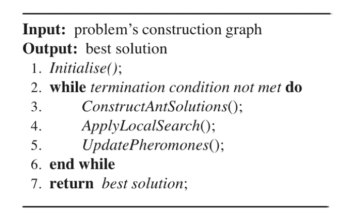
In the following figure, we present the pseudocode of a basic ACO algorithm which is composed of four primary procedures.
- Initialize: In this procedure, we initialize the algorithm’s parameters, the amount of pheromones, and the heuristic information relevant to the vertices and edges of the construction graph.
- Construct Ant Solution: In this procedure, we simulate the movement of artificial ants to gradually construct the candidate solutions. These ants navigate through the construction graph and make decisions at each step by applying a stochastic decision policy that incorporates the heuristic and pheromone information.
- Apply local search: The application of local search is optional and it facilitates us to refine ant’s solution. Local search would introduce minor adjustments to a solution to examine its neighbor solutions and the implementation of this algorithm usually exhibits great enhancement in the ACO algorithm’s performance.
- Update pheromones: In this procedure, we would update the pheromone levels on the components of the problem’s construction graph. The update involves either an increase as ants deposit pheromones along the paths while forming their candidate solutions, or a decrease due to the evaporation of pheromones.
We would iterate through the constructing and updating steps until we meet the termination criteria, at which point we are able to achieve the optimal solution.
Example
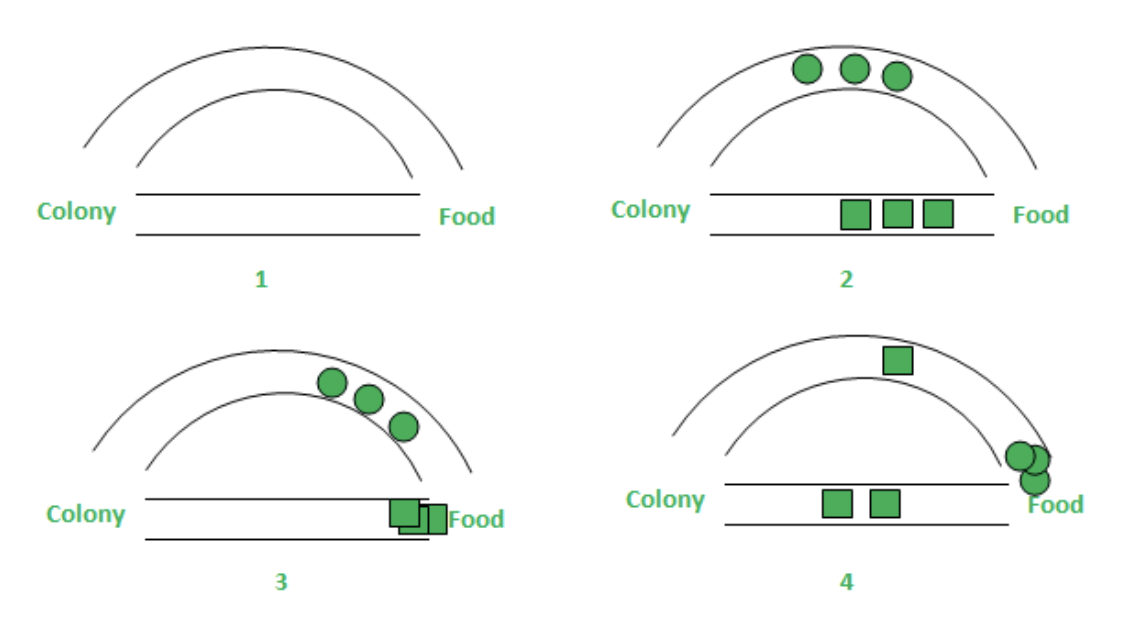
Here, we present a simple example of an ACO algorithm with one colony and one food source. The colony and food sources are connected by two paths with different lengths.
- At the first stage, all ants are located in their nest and there are no pheromone trails present on any path.
- Next, in the second stage, ants start from their nest to explore the food source with an equal probability of choosing either path (three ants choose the shorter path, and the other three choose the longer path). As they travel, ants deposit pheromones along their chosen path.
- Then, ants who choose the shorter path (represented by square points in the figure) arrive at the food source earlier.
- Arrived ants need to decide their return path back to their colony presented in stage 4. Since the pheromone trail of the shorter path has been formulated, the probability for ants to choose the shorter path would be higher than for them to choose the longer path (two ants choose to follow the shorter path and one ant chooses to follow the longer path).
More ants would increasingly favor the shorter path due to the aggregation of pheromones. The pheromone trail on the shorter path would increasingly be more attractive for ants. Moreover, the pheromone concentration for the longer path would gradually reduce due to evaporation which would decrease the probability for the following ants to select it.
For each iteration, the ants originally stay at their colony which denotes $V_s$, and move from their colony to explore the food source $V_d$ and return. Assuming two edges (paths) are $E_1$ and $E_2$ with corresponding lengths $L_1$ and $L_2$. In our example, we would denote $E_1$ as the shorter path and $E_2$ as the longer path which indicates that $L_1 < L_2$. In addition, the pheromone values for the two paths are $R_1$ and $R_2$.
The probability for each ant’s path selection would be $P_i=\frac{R_i}{R_1+R_2}$. If $R_1 > R_2$, the probability of choosing $E_1$ (path 1) would be higher than the probability of choosing $E_2$ (path 2) and vice-versa. As time goes on, the pheromone concentration level of a path would either increase due to the aggregation of pheromone as ants select to take this path or decrease due to the evaporation of pheromone.
The updation of pheromone concentration level on the path can be expressed as
Aggregation:
\[R_i=R_i+\frac{K}{L_i}\]K = A constant that determines the total amount of pheromone deposited by each ant.
Evaporation:
\[R_i=(1-v) \cdot R_i\]$v \in (0, 1]$ represents the pheromone evaporation rate.
Ant Colony Decision Trees (ACDT)
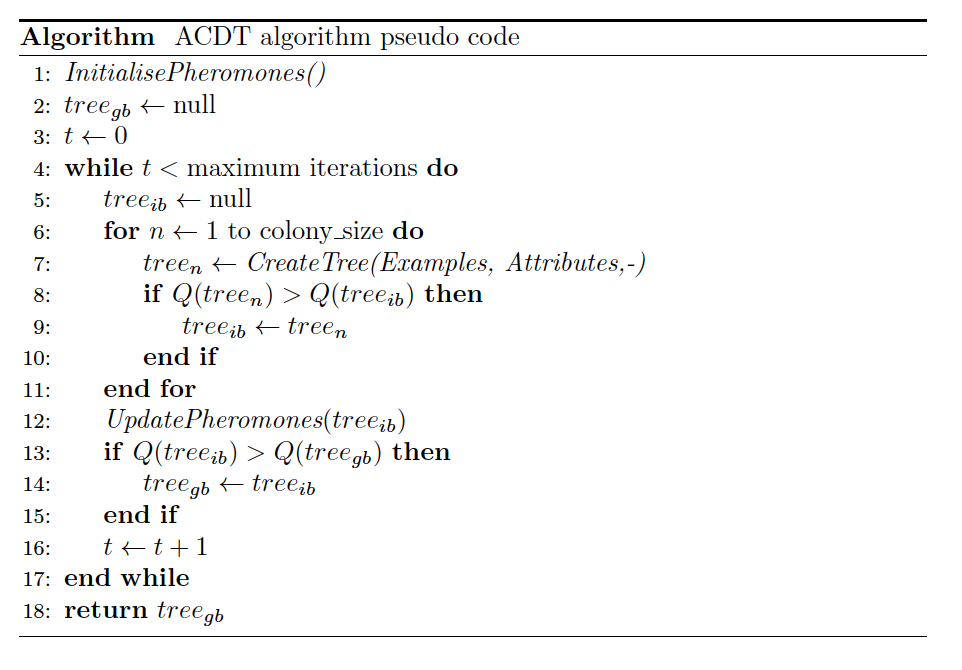
Based on the structure of the ACO algorithm, researchers have proposed applying it to decision tree modeling. As a result, a new metaheuristics approach based on ant colony algorithms, known as Ant Colony Decision Trees (ACDT), has been developed. Compared to the general decision tree algorithm, in ACDT, each ant chooses the appropriate attribute for splitting in each decision node of the constructed decision tree according to the heuristic function and pheromone values. Following the logic of ACO, the algorithm for ACDT can be written as below.
As can be seen in Figure 3, the algorithm starts by initializing the pheromone values and computing the heuristic information for each attribute of the training set. Then, it enters an iterative for loop. In each iteration, an ant in the colony creates a new decision tree until the maximum number of iterations is reached.
Each ant creates a decision tree (for loop) in a top-down fashion by probabilistically selecting attributes to be added as decision nodes based on the amount of pheromone and heuristic information. The procedure for creating a decision tree (CreateTree procedure) involves three parameters: the collection of training examples, the predictor attributes, and the edge that the ant is following, which initially corresponds to the default edge (indicated by the symbol ‘-‘). Once the tree construction procedure has finished, the created tree is pruned in order to simplify the tree and thus potentially avoid overfitting the model to the training data.
After the pruning, the tree is evaluated and if the quality of the newly pruned tree surpasses the quality of the existing iterative optimal tree, the iterative optimal tree (treeib) is updated. Finally, the iteration-best tree constructed by the ants is used to update the pheromone values, the global-best tree (treegb) is updated and a new iteration of the algorithm starts. When the maximum number of iterations is reached the global-best tree is returned as the discovered decision tree.
Example
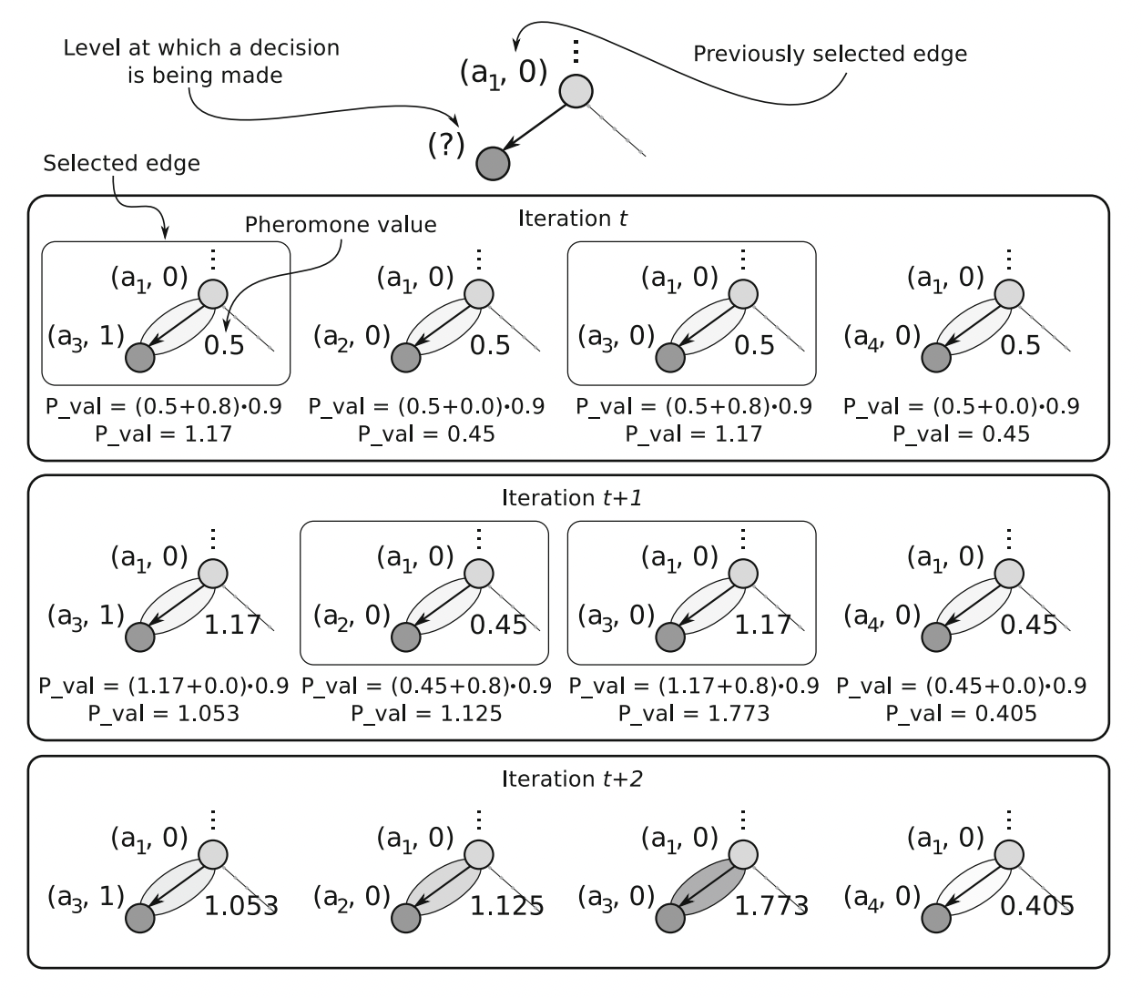
To better understand ACDT, we can look at the example below. In our example, ${a_1, a_2, a_3, a_4}$ are all possible binary attributes that we want to split on. The notation $(a_i,0)$ indicates that we choose to split on the attribute $a_i$ and go along the edge 0. For the ACDT algorithm, in which the pheromone trail is laid on the edges, pheromone trail values are assigned to edges between parent-child pairs of nodes.
We choose the evaporation rate $v$ to be 0.1. A higher value of this parameter leads to faster pheromone evaporation and higher punishment on the pheromone value. We assume that the initial pheromone value for all edges (trails) is 0.5, and once the ants select an edge, they leave an additional 0.8 amount of pheromone value.
- First, we assume that we split on attribute $a_1$, and go along with edge 0 in the previous iteration. That is, in this example, we begin with $(a_1, 0)$.
-
Then, in iteration t, two ant agents explore their possible paths based on an initial pheromone value equal to 0.5. One of the ants chooses $(a_3,1)$ and the other ant chooses $(a_3,0)$. After choosing these two edges, they leave 0.8 amount of pheromone on the edges, and the pheromone values on these two edges are updated to $(0.5+0.8) \times 0.9=1.17$. i.e., the amount of pheromone on the edges multiplied by (1 - evaporation rate). The unselected edges have no additional 0.8 pheromones and are therefore equal to $(0.5+0.0) \times 0.9 = 0.45$.
- Next, in iteration t+1, the two ant agents make the decision to move again, but based on the updated pheromone values, which are now ${1.17, 0.45, 1.17, 0.45}$. This time, one chooses $(a_2,0)$ and the other chooses $(a_3,0)$. Similar to the previous iteration, the pheromone values for the two newly chosen edges are updated to $(0.45 + 0.8) \times 0.9 = 1.125$ and $(1.17 + 0.8) \times 0.9 = 1.773$
- The above process continues until the maximum number of iterations is reached. Eventually, the greater the pheromone trail value, the more ant agents have chosen a given solution.
We can see that in such a trivial case after two algorithm iterations two edges that were once included in the previously constructed best decision trees (with the same quality) have different values of the pheromone trail. Edge $((a_1, 0), (a_3, 1), 1.053)$, which occurred earlier, has a smaller value of the pheromone trail than edge $((a_1, 0), (a_4, 0), 1.125)$, which occurred later. This shows that, unlike the greedy decision tree algorithm, ACDT, in collaboration with ACO, aims to find the global optimum through iterative improvement and collective learning from the experience of multiple ant agents, thus helping to improve prediction accuracy.
Reference
Boryczka, U., & Kozák, J. (2010). Ant colony decision trees – a new method for constructing decision trees based on ant colony optimization. In Lecture notes in computer science (pp. 373–382). https://doi.org/10.1007/978-3-642-16693-8_39
Otero, F. E. B., B., Freitas, A. A., Johnson, C. G., & School of Computing, University of Kent, UK. (2012). Inducing Decision Trees with an Ant Colony Optimization Algorithm. Applied Soft Computing. https://doi.org/10.1016/j.asoc.2012.05.028
Hafeez, M. A., Rashid, M., Tariq, H., Abideen, Z. U., Alotaibi, S. S., & Sinky, M. H. (2021). Performance improvement of Decision Tree: a robust classifier using Tabu search algorithm. Applied Sciences, 11(15), 6728. https://doi.org/10.3390/app11156728
GeeksforGeeks. (2020, May 17). Introduction to Ant Colony Optimization. GeeksforGeeks. https://www.geeksforgeeks.org/introduction-to-ant-colony-optimization/